Improving Prediction Accuracy
Prediction Using a Geographically Restricted List
pybioclip provides three features for making predictions using a restricted set of terms:
--cls--bins--subset
One way to populate the restricted set of terms is to use taxa that are known to have been observed in a specific geographic region.
There are many ways to obtain a list with this constraint. Two noteworthy methods are:
- Using the Global Biodiversity Information Facility (GBIF) to download a list of taxa that have been observed in a specific geographic region.
- Using Map of Life (MOL) to download a list of taxa that have been observed in a specific geographic region.
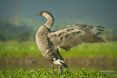
In our examples, we will use the image below of the nēnē, or the Hawaiian goose (Branta sandvicensis). Its full taxonomic classification is Animalia Chordata Aves Anseriformes Anatidae Branta sandvicensis.
Save this image to your working directory as nene.jpg for the example.
Getting a Geographically Restricted List of Taxa
Both GBIF and MOL provide web interfaces that enable users to produce a species list filtered by geographic coordinates and regions. A brief tutorial is provided. These examples illustrate a small subset of the capabilities provided by these platforms.
GBIF Web Interface Tutorial
You must have an account with GBIF to create downloads with a DOI. You do not need an account to download data with a DOI created by others.
Visit https://www.gbif.org/ and click Login and Register to create an account.
Once you have an account, log in to manage data downloads from your profile.
Example: filter for all occurrences of birds in the islands of Hawai'i with GBIF.
Note
Rather than creating a new download, you may use https://doi.org/10.15468/dl.469rtz, which was prepared for this example using the steps below. The information in this download may be different from a download you create, as more data is being added to GBIF regularly. Taxa have been extracted from the species list in this download and are available in:
- hawaii_bird_species_list.txt
- hawaii_bird_families_list.txt
- hawaii_bird_family_bins_list.csv (terms for bins of families were created manually)
You can save these files to your working directory for the example.
- Log in to https://www.gbif.org/ and click
OCCURRENCESnear the search bar. - Apply filters for your search (you can apply the filters in any combination and order).
- To filter by region, use
LocationwithIncluding coordinates,Administrative areas (gadm.org),Country or area, orContinent. - The
Locationfeature is very flexible. You may use the built-in map widget to specify one or more regions with polygons or squares by hand. You may also specify one or more square ranges by entering precise coordinates intoRangeand/orGeometry. These features are able to be used in combination. - Under the
Scientific namefilter, type "Aves", and select "Aves Class" from the search results. - Under the
Locationfilter, clickGeometry, and enter the following into the "WKT or GeoJSON" field to specify the main eight islands of Hawai'i:POLYGON((-160.54 18.54, -154.46 18.54, -154.46 22.26, -160.54 22.26, -160.54 18.54))- You could also paste the equivalent raw content of the file hawaii.geojson into the "WKT or GeoJSON" field under
Geometry.
- You could also paste the equivalent raw content of the file hawaii.geojson into the "WKT or GeoJSON" field under
- Click
ADD
- To filter by region, use
- Download the data.
- Once the query completes, click
DOWNLOAD. - Select the
SPECIES LIST, read and agree to the terms of use, and clickUNDERSTOOD. - The download will be prepared and associated with the DOI displayed at the top of the page, and you will receive an email when it is ready.
- The CSV will contain a list of taxa that meet the requirements of the filter with contents as defined by the GBIF "Species list" download format.
- You may extract contents of the CSV to a text file as you see fit for use with
pybioclip, as we have withhawaii_bird_species_list.txt,hawaii_bird_families_list.txt, andhawaii_bird_family_bins_list.csv.
- Once the query completes, click
MOL Web Interface Tutorial
There are no prerequisites. An account with MOL is optional and not required for downloading data.
Note that any URL shared for a filter applied to MOL will yield filter results as of the date the URL is used (rather than the date you applied the filter). You should host your own copy of the data if you need to ensure the data is static.
Example: filter for all species of birds in the islands of Hawai'i with MOL.
- Visit https://mol.org/ and click
Regions. - Under "Search for an area by name:", type "Hawai'i" and select "Hawai'i, United States".
- Click
Go to Species Report. This should take you to a page matching this URL. - Under "Species", click
<N> Birds, where<N>is the number of bird species in the region. This should append&group=birdsto the URL. - Refresh the browser to apply the Birds filter to the download. The filter will be applied when loading the URL with the Birds filter applied. Note that if you download before refreshing, the download will include all species in the region.
- Click
Download, review the information in the pop-up about the download contents, and clickDownload Now.
Examples Using a Geographically Restricted List of Taxa for Prediction
These examples use the files containing information extracted from the GBIF download. You are encouraged to practice by creating similarly formatted files with the scientific_name and family columns from the SpeciesList.csv file in the MOL download.
Example: Predict the species of an image using open-ended classification.
bioclip predict --k 5 --format table nene.jpg
+-----------+----------+----------+-------+--------------+----------+--------+-----------------+---------------------+----------------+---------------------+
| file_name | kingdom  |  phylum  | class |    order     |  family  | genus  | species_epithet |       species       |  common_name   |        score        |
+-----------+----------+----------+-------+--------------+----------+--------+-----------------+---------------------+----------------+---------------------+
|  nene.jpg | Animalia | Chordata |  Aves |  Gruiformes  | Gruidae  |  Grus  |       grus      |      Grus grus      |  Common Crane  |  0.7501388788223267 |
|  nene.jpg | Animalia | Chordata |  Aves |  Gruiformes  | Gruidae  |  Grus  |     communis    |    Grus communis    |                | 0.07198520749807358 |
|  nene.jpg | Animalia | Chordata |  Aves | Anseriformes | Anatidae | Branta |   sandvicensis  | Branta sandvicensis | Hawaiian Goose | 0.04125870019197464 |
|  nene.jpg | Animalia | Chordata |  Aves |  Gruiformes  | Gruidae  |  Grus  |     cinerea     |     Grus cinerea    |                | 0.03031359612941742 |
|  nene.jpg | Animalia | Chordata |  Aves |  Gruiformes  | Gruidae  |  Grus  |     monacha     |     Grus monacha    |  Hooded Crane  | 0.02994249388575554 |
+-----------+----------+----------+-------+--------------+----------+--------+-----------------+---------------------+----------------+---------------------+
Incorrect top predictions.
The top two predictions are incorrect. This suggests that filtering the possibilities for predicted labels may improve the accuracy of the predictions.
We can imagine that all we know about the image is that it was taken on one of the Hawaiian islands. We can use multiple approaches incorporating the geographically restricted lists to make a more informed decision.
Example: Predict the species of an image using the geographically restricted list of species directly as custom labels.
Using hawaii_bird_species_list.txt:
bioclip predict --k 3 --format table --cls hawaii_bird_species_list.txt nene.jpg
+-----------+---------------------+---------------------+
| file_name |    classification   |        score        |
+-----------+---------------------+---------------------+
|  nene.jpg | Branta sandvicensis |  0.7710946798324585 |
|  nene.jpg |    Rhea americana   | 0.10109006613492966 |
|  nene.jpg |   Branta leucopsis  |  0.0416080504655838 |
+-----------+---------------------+---------------------+
- Prediction accuracy: The predictions are more accurate because they are limited to species that are known to be present in the geographic region.
Disadvantages of this approach:
- Performance: The prediction is slow because the embeddings must be calculated for all species in the list. See the following examples for approaches to speed up prediction.
- Potential misses: The predictions are limited to the species in the list, which may not include the correct species if it is an anomalous occurrence.
Example: Predict the species of an image by combining the geographically restricted list with the precomputed embeddings of the TOL subset of taxa.
Obtain the TOL subset.
bioclip list-tol-taxa > tol_subset.csv
Filter the TOL subset to include only the geographically restricted list in hawaii_bird_species_list.txt. For example, with Pandas in Python:
import pandas as pd

# Load the TOL subset.
df_tol = pd.read_csv('tol_subset.csv')

# Load the list of species.
df_species = pd.read_csv('hawaii_bird_species_list.txt', header=None, names=['species'])

# Merge the TOL subset with the list of species, inner merge
df_merged = pd.merge(df_tol, df_species, on='species')

# Save the merged list to a file to use with the --subset option.
df_merged["species"].to_csv("tol_subset_species_filtered.csv", index=False, header=True)
Predict using the filtered TOL subset.
bioclip predict --k 3 --format table --subset tol_subset_species_filtered.csv nene.jpg
+-----------+----------+----------+-------+--------------+----------+--------------+-----------------+---------------------+------------------+---------------------+
| file_name | kingdom  |  phylum  | class |    order     |  family  |    genus     | species_epithet |       species       |   common_name    |
score        |
+-----------+----------+----------+-------+--------------+----------+--------------+-----------------+---------------------+------------------+---------------------+
|  nene.jpg | Animalia | Chordata |  Aves | Anseriformes | Anatidae |    Branta    |   sandvicensis  | Branta sandvicensis |  Hawaiian Goose  |  0.7040964365005493 |
|  nene.jpg | Animalia | Chordata |  Aves |  Rheiformes  | Rheidae  |     Rhea     |    americana    |    Rhea americana   |   Greater Rhea   | 0.18546675145626068 |
|  nene.jpg | Animalia | Chordata |  Aves |  Gruiformes  | Gruidae  | Anthropoides |      virgo      |  Anthropoides virgo | Demoiselle Crane | 0.04178838059306145 |
+-----------+----------+----------+-------+--------------+----------+--------------+-----------------+---------------------+------------------+---------------------+
Advantages of this approach:
- Performance: Significant speedup in prediction time because the embeddings are precomputed.
- Prediction accuracy: The predictions are more accurate than open-ended prediction alone because they are limited to species that are known to be present in the geographic region.
Disadvantages of this approach:
- Potential misses: Only taxa in the TOL subset can be included in the geographically restricted list, which may exclude entries present in the external list.
Example: Predict the species of an image combining open-ended classification with the geographically restricted list using custom labels.
This approach will produce two outputs, an unconstrained open-ended prediction and a prediction constrained by the geographically restricted list for comparison.
Predict the top 20 species with open-ended classification, saving the predictions to a file.
bioclip predict --k 20 nene.jpg > bioclip_species_predictions_oe.csv
import pandas as pd

# Load the open-ended predictions.
df_predictions = pd.read_csv('bioclip_species_predictions_oe.csv')

# Load the geographically restricted list of species.
df_hawaii_species = pd.read_csv('hawaii_bird_species_list.txt', header=None, names=['species'])

# Filter the predictions to include only species in the geographically restricted list.
df_merged = pd.merge(df_predictions, df_hawaii_species, on='species', how='inner')

# Save the filtered list to a file to use with the --cls option.
df_merged["species"].to_csv("bioclip_species_predictions_filtered.txt", index=False, header=False)
Predict the species using the filtered list.
bioclip predict --k 3 --format table --cls bioclip_species_predictions_filtered.txt nene.jpg
+-----------+---------------------+---------------------+
| file_name |    classification   |        score        |
+-----------+---------------------+---------------------+
|  nene.jpg | Branta sandvicensis |  0.8363304734230042 |
|  nene.jpg |    Rhea americana   | 0.10964243859052658 |
|  nene.jpg |   Anser cygnoides   | 0.02564687840640545 |
+-----------+---------------------+---------------------+
- Anomaly detection: In the case of an anomalous occurrence--a true sighting of an organism that has not been recorded in that region previously--we have BioCLIP's first best guess handy in
bioclip_species_predictions_oe.csv, which is not constrained by the geographical list. This may be useful for flagging a novel invasive species or otherwise undocumented sighting. - Performance: The long geographically restricted list is reasonably pruned, which speeds up prediction, giving
bioclip_species_predictions_filtered.txt. - Balanced approach: This may be a good balanced approach if there is uncertainty about the origin of the organism in the image.
Disadvantages of this approach:
- Potential misses: The primary filter is the open-ended classification, which may not include the correct prediction if
-kis set too low or in challenging cases.
Example: Predict the family of an image among bird families in Hawai'i as custom labels.
Using hawaii_bird_families_list.txt:
bioclip predict --k 3 --format table --cls hawaii_bird_families_list.txt nene.jpg
+-----------+----------------+---------------------+
| file_name | classification |        score        |
+-----------+----------------+---------------------+
|  nene.jpg |    Anatidae    | 0.34369930624961853 |
|  nene.jpg |   Ciconiidae   | 0.28970828652381897 |
|  nene.jpg |    Gruidae     | 0.17063161730766296 |
+-----------+----------------+---------------------+
Example: Predict a custom binned classification of an image using the binned list of families.
Using hawaii_bird_family_bins_list.csv:
bioclip predict --k 3 --format table --bins hawaii_bird_family_bins_list.csv nene.jpg
+-----------+-----------------------+---------------------+
| file_name |     classification    |        score        |
+-----------+-----------------------+---------------------+
|  nene.jpg |       Waterfowl       |  0.3437104821205139 |
|  nene.jpg | Shorebirds/Waterbirds |  0.3415525555610657 |
|  nene.jpg |         Cranes        | 0.17063717544078827 |
+-----------+-----------------------+---------------------+
Example: Predict the order rank of an image by combining the geographically restricted list with the precomputed embeddings of the TOL subset of taxa.
This example is similar to the earlier example using the TOL subset, but using a higher taxonomic rank with this approach has some considerations to keep in mind, as we will explore.
This example also requires you to preprocess a list of custom labels yourself.
To do so, download the GBIF filtered species list prepared at https://doi.org/10.15468/dl.469rtz. Extract the file 0001260-250123221155621.csv to your working directory. Note that the delimiter in this file is the tab character (\t).
Retrieve the TOL subset.
bioclip list-tol-taxa > tol_subset.csv
0001260-250123221155621.csv. For example, with Pandas in Python:
import pandas as pd

# Load the TOL subset.
df_tol = pd.read_csv('tol_subset.csv')

# Load the CSV from GBIF containing taxonomic data of bird species in Hawai'i.
df_gbif = pd.read_csv('0001260-250123221155621.csv', delimiter='\t')

# Filter the GBIF list to include only bird orders.
df_gbif_orders = df_gbif['order'].drop_duplicates()

# Merge the orders from the TOL subset with the orders from GBIF. inner merge
df_merged = pd.merge(df_tol, df_gbif_orders, on='order', how='inner')

# Save the merged list to a file to use with the --subset option.
df_merged["order"].drop_duplicates().to_csv("tol_subset_orders_filtered.csv", index=False, header=True)
Predict using the filtered TOL subset.
bioclip predict --k 3 --format table --subset tol_subset_orders_filtered.csv nene.jpg
+-----------+----------+----------+-------+--------------+----------+--------+-----------------+---------------------+----------------+---------------------+
| file_name | kingdom  |  phylum  | class |    order     |  family  | genus  | species_epithet |       species       |  common_name   |
    score        |
+-----------+----------+----------+-------+--------------+----------+--------+-----------------+---------------------+----------------+---------------------+
|  nene.jpg | Animalia | Chordata |  Aves |  Gruiformes  | Gruidae  |  Grus  |       grus      |      Grus grus      |  Common Crane  |  0.7614361047744751 |
|  nene.jpg | Animalia | Chordata |  Aves |  Gruiformes  | Gruidae  |  Grus  |     communis    |    Grus communis    |                | 0.07306931912899017 |
|  nene.jpg | Animalia | Chordata |  Aves | Anseriformes | Anatidae | Branta |   sandvicensis  | Branta sandvicensis | Hawaiian Goose | 0.04188006371259689 |
+-----------+----------+----------+-------+--------------+----------+--------+-----------------+---------------------+----------------+---------------------+
Incorrect top predictions: when not to use --subset to speed up prediction.
There are a few things to note about this output:
- The top predictions are incorrect as with the open-ended classification example.
- The prediction is specified to the species rank though our
--subsetfile contains orders. This is expected behavior.- All of the species (and orders) that are not known by GBIF to be present in Hawai'i are excluded from
tol_subset_orders_filtered.csv--however, filtering by higher-rank taxa does not eliminate non-local species. That is, even though Grus grus and Grus communis (members of order Gruiformes, i.e. "crane-like") are not found in Hawai'i, other members of the order Gruiformes are found in Hawai'i according to GBIF. Since the--subsetmethod predicts to species level, these species are included in the prediction. - In other words, if just one species of a higher-rank taxon is found in the geographic region, all species of that taxon will be included in the prediction when using
--subset.
- All of the species (and orders) that are not known by GBIF to be present in Hawai'i are excluded from
- In this case, it is not advisable to use higher taxa in the geographically restricted list for use with
--subsetwithout additional filtering.
If you know that the organism in your image is not from the order Gruiformes (and others), you can exclude that term (and others) from the filtered list. This will improve the accuracy of the predictions.
In Python:
# Following the merge step between the TOL subset and the GBIF orders, remove the term Gruiformes from the list.
df_merged = df_merged[df_merged['order'] != 'Gruiformes']

# Save the filtered list to a file to use with the --subset option.
df_merged["order"].drop_duplicates().to_csv("tol_subset_orders_filtered.csv", index=False, header=True)
bioclip predict --k 3 --format table --subset tol_subset_orders_filtered.csv nene.jpg
+-----------+----------+----------+-------+--------------+-------------+--------------+-----------------+-----------------------+----------------+---------------------+
| file_name | kingdom  |  phylum  | class |    order     |    family   |    genus     | species_epithet |        species        |  common_name   |        score        |
+-----------+----------+----------+-------+--------------+-------------+--------------+-----------------+-----------------------+----------------+---------------------+
|  nene.jpg | Animalia | Chordata |  Aves | Anseriformes |   Anatidae  |    Branta    |   sandvicensis  |  Branta sandvicensis  | Hawaiian Goose |  0.4851439893245697 |
|  nene.jpg | Animalia | Chordata |  Aves |  Rheiformes  |   Rheidae   |     Rhea     |    americana    |     Rhea americana    |  Greater Rhea  | 0.12779226899147034 |
|  nene.jpg | Animalia | Chordata |  Aves | Galliformes  | Phasianidae | Tetraogallus |     altaicus    | Tetraogallus altaicus | Altai Snowcock | 0.10936115682125092 |
+-----------+----------+----------+-------+--------------+-------------+--------------+-----------------+-----------------------+----------------+---------------------+
It could be sensible to use --subset with higher taxa if:
- You want to speed up predictions by using precomputed embeddings.
- You are confident that the species in the higher taxa are all found in the filtered list of higher taxa labels (e.g. if you know it belongs to a certain order but some other order has species that look confusingly similar, you can exclude the other order from the list).