Mind the Tail: Data Selection Through Sparse Concepts

Zhang, Ziheng; Hulkund, Neha; Lee, Colin; Mai, Zheda; Shen, Hui; Ding, Ying; Berger-Wolf, Tanya; Beery, Sara; Chao, Wei-Lun; Gu, Jianyang

Concept-Based Data Selection

Mind the Tail

Data Selection Through Sparse Concepts

Ziheng Zhang^1,2†· Neha Hulkund³· Colin Lee²· Zheda Mai²· Hui Shen⁴
Ying Ding¹· Tanya Berger-Wolf²· Sara Beery³· Wei-Lun Chao⁵· Jianyang Gu^2,3†

¹University of Texas at Austin ²The Ohio State University ³Massachusetts Institute of Technology ⁴University of Michigan ⁵Boston University

Paper Code arXiv Models & Data Contact Cite

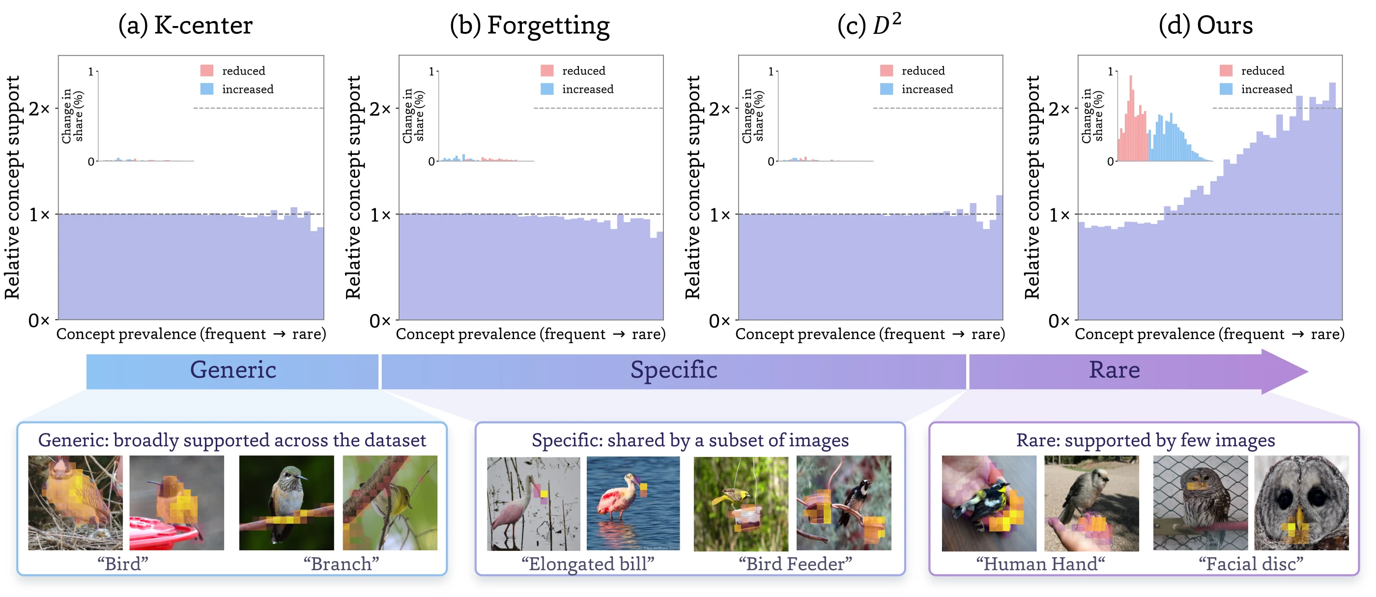
A training subset determines how much support each visual concept gets, from objects and attributes to textures and backgrounds. Tail concepts appear in only a few images and are easy to lose when data is reduced, which can hurt test-time robustness. We use sparse-autoencoder concepts to make this allocation explicit and shift more support toward the tail.

Method We accumulate each concept's support as images are selected. Diminishing returns lower the value of concepts that are already well covered, and local support favors samples that, together with their neighbors, contribute to under-supported concepts, so recurring underrepresented concepts are preferred over isolated occurrences.
Finding Test images with concepts that gained support improve the most. Broader coverage of the tail, including context unrelated to the class, also improves robustness to out-of-distribution and spurious contexts.
Results Improvements over strong data selection baselines on fine-grained, spurious-correlation, and general image classification, and on CLIP pretraining with CC12M, with the largest margins at small budgets.

Method

From Concept Value to Sample Value

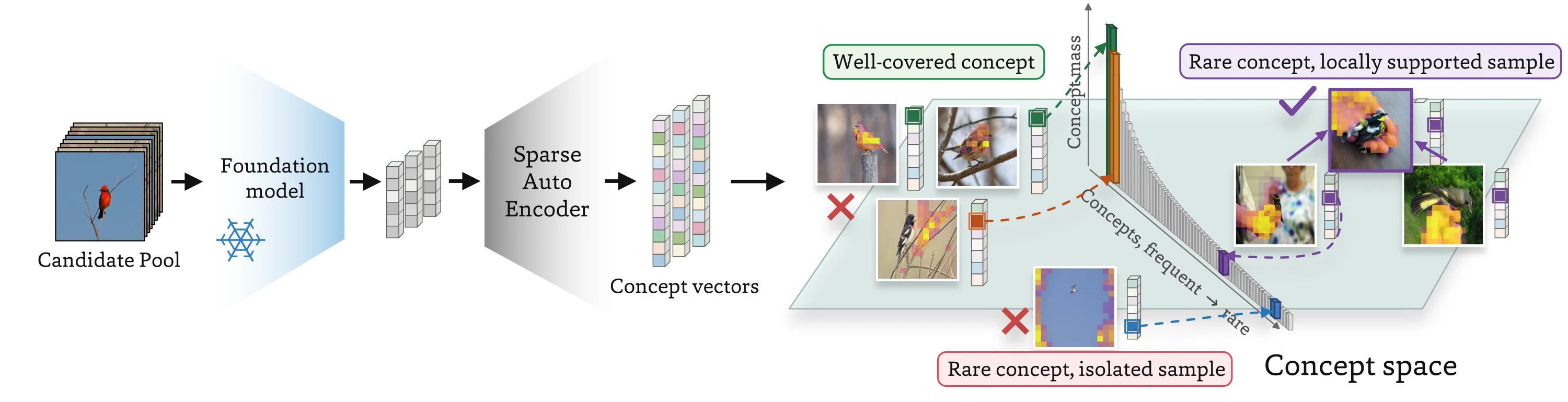
We measure concept coverage to find what evidence the subset still needs, and local support to decide which samples fill that gap.

Pipeline: candidate images pass through a frozen foundation model and a sparse autoencoder to produce concept vectors. In concept space, a sample with a well-covered concept and an isolated sample with a rare concept are rejected, while a locally supported sample with a rare concept is selected. — **Overview.** SAEs turn foundation-model patch features into sparse concept vectors, and we track the support each concept has in the subset. The objective favors samples whose under-supported concepts are also carried by their neighbors, over samples that only add head concepts or sit alone in a rare region.

Step 1

Describe each image by its sparse concepts

An SAE with $C$ dimensions on DINOv3 patch features, max-pooled per image, gives a sparse concept vector $\mathbf{x}_i$, where $\mathbf{x}_i[c]$ is the activation of concept $c$.

SAE concepts follow a long-tailed distribution. Fine-grained attributes, uncommon objects, and context variations appear in only a few images, which makes them easy to lose when data is reduced.

Image $I_i$ DINOv3 patches SAE max-pool $\mathbf{x}_i \in \mathbb{R}^{C}$

Dimensions tend to fire on recurring visual patterns, such as a bill shape, a feeder, a hand, or a sky background.

Step 2

Concept coverage: where is support missing?

As images are added, we accumulate each concept's support and apply diminishing returns. Well-covered concepts become worth less, so under-supported ones become more competitive. The objective needs no explicit definition of the tail or a target frequency.

$$F(\mathcal{S}) \;=\; \sum_{c=1}^{C} \log\!\Big(1 + \sum_{I_i \in \mathcal{S}} \mathbf{x}_i[c]\Big)$$

The concave $\log(1+\cdot)$ saturates head concepts and leaves room for the tail.

Step 3

Local support: which samples fill the gap?

Rare concepts do not automatically dominate selection, because the samples that carry them may receive limited local support when isolated. Each candidate also receives complementary credit for concepts recurring among nearby samples, so recurring underrepresented concepts are favored over isolated occurrences.

$$\tilde{\mathbf{x}}_i[c] \;=\; \mathbf{x}_i[c] \;+\; \beta \!\!\sum_{t:\, I_i \in \mathcal{N}_k(t)}\!\! a_{ti}\, \mathbf{x}_t[c]$$

$\mathcal{N}_k(t)$: the $k$ nearest neighbors of $I_t$ in SAE space; $a_{ti}$: cosine similarity normalized over the neighbors; $\beta$: strength of local support.

Analysis

Which Concepts Does a Subset Support?

Do different selectors change the concept distribution, and do the concepts that gain support matter downstream?

FindingDifferent criteria, similar concept profiles

We profile each NABirds subset by how many concepts it covers, how evenly it spreads activation mass, and how common its concepts are relative to the full dataset.

K-Center, Forgetting, and D²-Pruning end up close to random sampling on all three measures, while our subset moves noticeably more support to tail concepts.

Method	Unique coverage	Effective number	Prevalence ratio
Random	7,973	865	1.00
K-Center	8,215	893	0.97
Forgetting	8,120	888	0.97
D²-Pruning	8,099	887	0.97
Ours	8,951	1,124	0.74

NABirds subsets. A prevalence ratio below 1 means more support for tail concepts.

Bar chart of accuracy gain over random selection for test images whose concepts were reduced, unchanged, or enhanced in training support, on NABirds and CC12M to ImageNet-1K linear probe. Enhanced concepts show the largest gains. — **Accuracy gain over random** on test images whose concepts lost, kept, or gained training support.

FindingEnhanced concepts improve the most

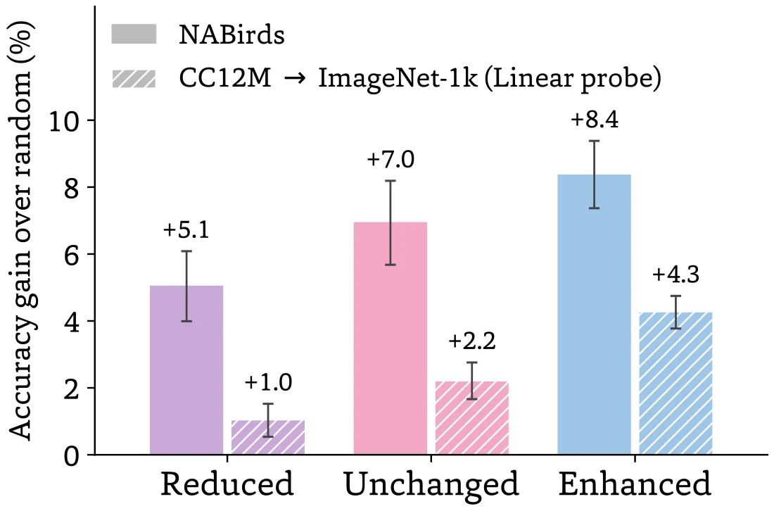
We group concepts by how their training support changed relative to random selection, then test on images where each concept is strongly active.

All three groups improve over random selection. Images with enhanced concepts improve the most, both on NABirds and on ImageNet-1K after CLIP pretraining.

Case Study · NABirds

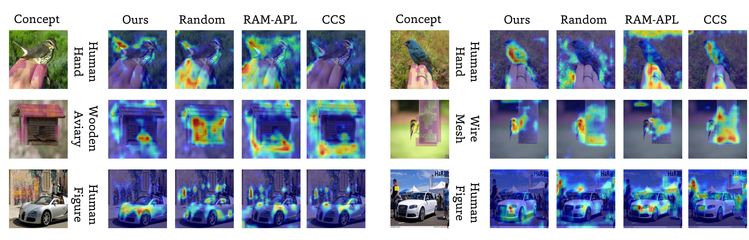
When the Tail Is Context: The “Human Hand” Concept

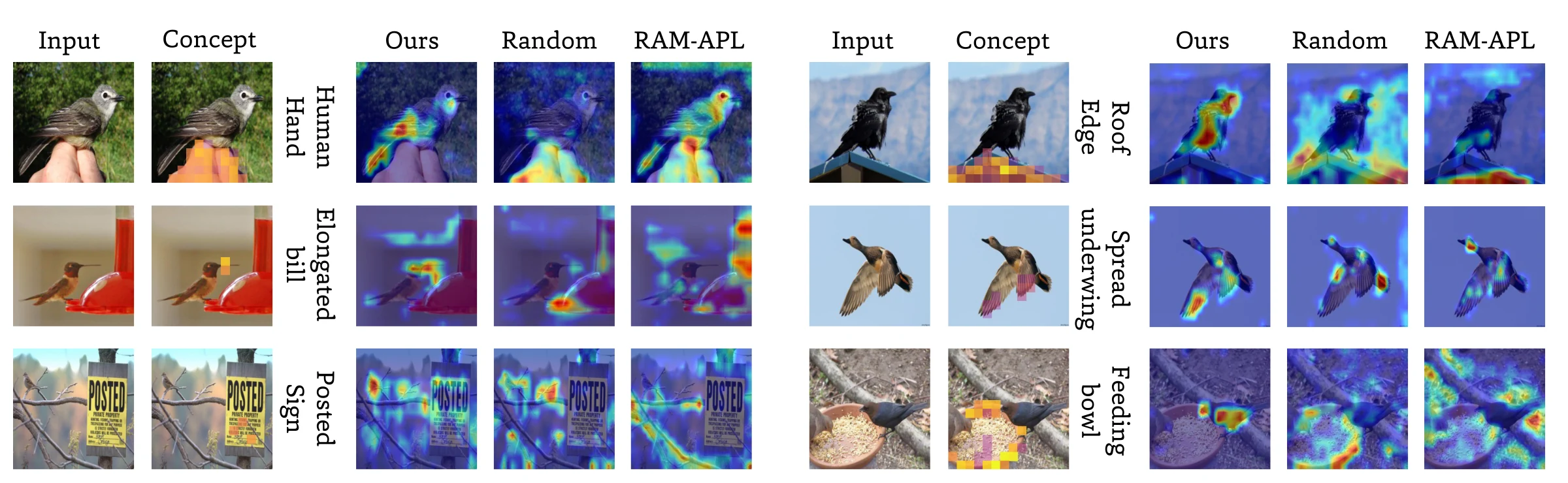
Some enhanced concepts are discriminative features, such as bills and wings. Others, such as hands, signs, and feeders, are not directly related to the species, and accuracy on test images with these concepts also improves.

Finer-CAM maps for test images with enhanced concepts: human hand, elongated bill, posted sign, roof edge, spread underwing, feeding bowl. Models trained on our subset focus on the bird; random and RAM-APL models often focus on the hand, sign, feeder, or bowl. — **Finer-CAM on enhanced concepts.** The model trained on our subset attends mostly to the bird, while the models trained on random and RAM-APL subsets put more weight on the hand, sign, or feeder.

Contextual concepts such as a hand carry little information about the species. Spreading them across more categories during training helps keep test images with that context in distribution and lowers the risk that the context becomes a shortcut for a few classes.

More Finer-CAM examples NABirds & Stanford Cars

Additional Finer-CAM attribution maps on NABirds and Stanford Cars comparing our method, Random, RAM-APL, and CCS. — **More Finer-CAM maps.** Across these examples, our model places more attribution on the object, while models trained on Random, RAM-APL, and CCS subsets more often attend to the surrounding context.

Case Study · Waterbirds

Broader Coverage and Background Shortcuts

In Waterbirds, bird type is spuriously correlated with the background. Our subsets contain more images that break this correlation.

FindingMore bias-conflicting images, without group labels

Bias-conflicting images, such as waterbirds on land, make up 18.8% of our subset, compared with under 10% for the other selectors we compare. Our method does not use group labels.

FindingGroup composition explains part of the gain

Random subsets with the same label-background counts close only part of the gap to our subset, and filling the same quotas with difficult images does worse. This suggests the improvement comes from both a more favorable group composition and richer visual evidence within each group.

Method	Counter-corr.	WGA ↑	All-bg ↑
Random	4.0	52.3	57.6
Forgetting	5.0	31.6	32.4
K-Center	5.4	57.5	72.6
Moderate	9.3	60.5	78.3
Ours	18.8	68.6	86.5
Group-matched controls (same label-background counts as ours)
Random	18.8	63.7	84.2
Difficult	18.8	52.2	73.7
Easy	18.8	64.0	85.8

Waterbirds (%). Counter-corr.: share of bias-conflicting images. WGA: worst-group accuracy. All-bg: correct under all four backgrounds.

Design Choices

Representation and Neighborhood Weight

We look at two design choices: which features to measure concept support with, and how much weight to give local support relative to coverage.

RepresentationSAE concepts give a clearer selection signal

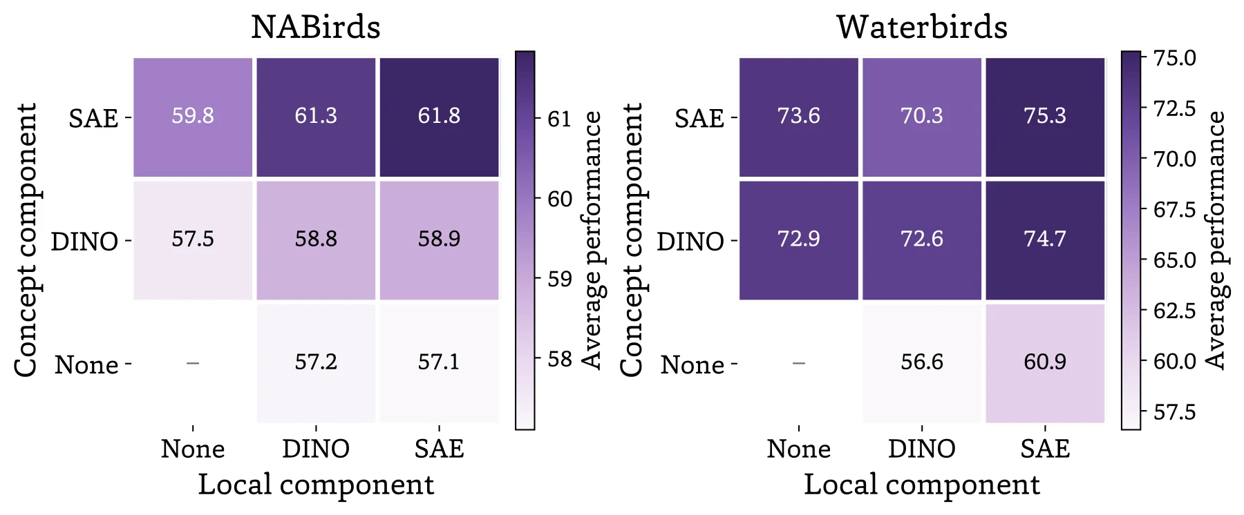
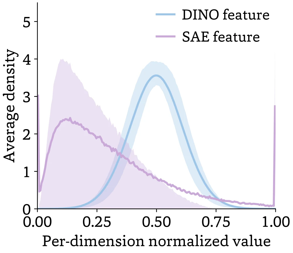
Heatmaps on NABirds and Waterbirds of average performance when concept coverage and local support are computed from SAE features, DINO features, or removed. SAE for both components is best or near best. — **Representation ablation.** Rows: features for concept coverage; columns: features for local support (*None* removes it).

Average per-dimension activation density: DINO features follow a single bell-shaped distribution, while SAE features show multiple peaks. — **Why SAEs help.** Per-dimension activation density of DINO vs. SAE features.

With the same objective, SAE features work best for concept coverage on NABirds, and moving local support from DINO to SAE space helps most on Waterbirds. DINO dimensions are roughly normally distributed across images, while SAE dimensions have multiple peaks, which separates images with different characteristics more clearly and gives the objective a more informative signal about accumulated and rare concepts. The method stays effective with concepts from other encoders (DINOv2, DINOv3-S/B, CLIP, SigLIP 2).

BalanceWeighting local support against coverage

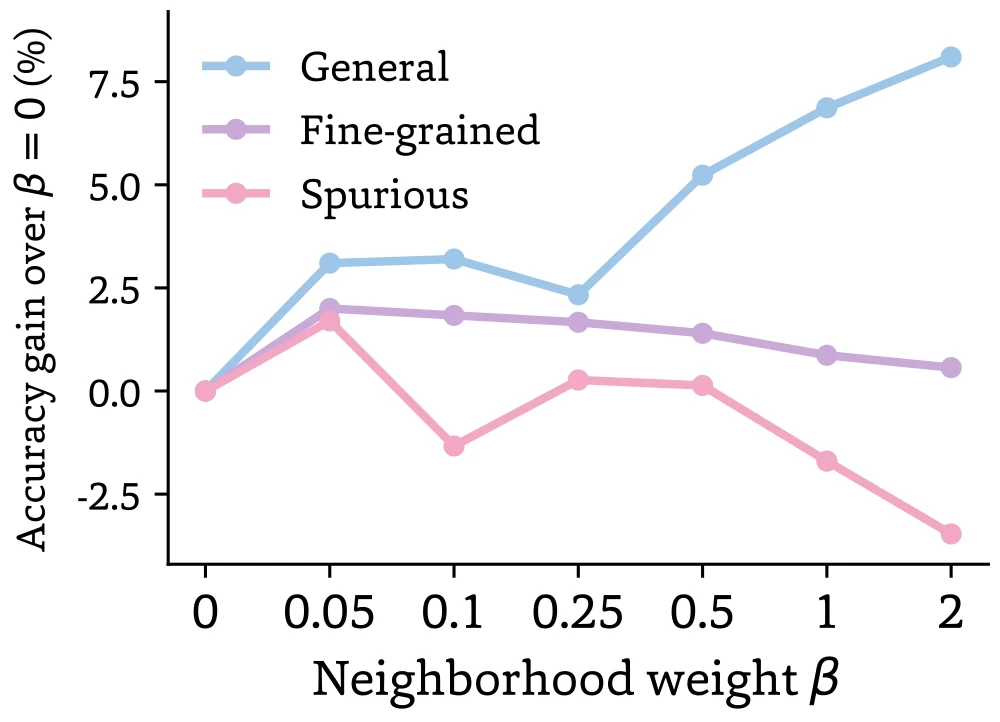
The weight $\beta$ controls how much local support counts relative to coverage. In all three settings we test, a small amount of local support ($\beta = 0.05$) improves over coverage alone.

Fine-grained and spurious-correlation datasets work best at $\beta = 0.05$, which keeps the emphasis on broad coverage. Tiny-ImageNet, a general dataset with a wider range of concepts, works best with much stronger local support ($\beta = 2$).

Accuracy gain over beta equals zero as a function of neighborhood weight beta for general, fine-grained, and spurious datasets. Fine-grained and spurious peak at small beta; general peaks at beta equals 2. — **Effect of $\beta$** on general (Tiny-ImageNet), fine-grained (NABirds), and spurious-correlation (Waterbirds) data.

Benchmarks

Benchmark Results

Our subsets give the best result at most budgets on NABirds, Stanford Cars, Waterbirds, and CLIP pretraining, with the largest margins at small budgets. On Spawrious, EL2N and CCS score higher at most budgets.

Image classification ResNet-50 trained on the selected subset

NABirds Accuracy

Method	10%	20%	30%	50%	70%
Random	35.6	55.3	64.9	73.3	77.1
K-Center	31.6	54.4	64.9	74.1	77.8
Forgetting	22.4	49.8	63.3	74.3	78.1
EL2N	16.8	44.4	61.2	74.4	78.5
Moderate	34.6	56.0	64.9	73.7	77.5
CCS	39.7	57.7	65.5	73.6	77.6
D²-Pruning	25.8	54.8	66.6	74.7	77.9
InfoMax	22.5	52.0	64.7	72.7	76.3
RAM-APL	39.3	54.7	61.7	69.8	74.8
SDM	37.5	56.3	64.5	73.7	78.2
Ours	42.9	59.4	67.4	75.2	78.3

Full dataset (100%): 80.3

Stanford Cars Accuracy

Method	10%	20%	30%	50%	70%
Random	21.9	45.2	63.1	78.0	83.7
K-Center	16.6	39.1	56.3	77.5	83.9
Forgetting	11.8	37.0	56.7	72.2	81.1
EL2N	8.9	28.4	49.2	71.0	79.3
Moderate	19.7	45.9	59.8	77.3	83.8
CCS	23.6	49.3	62.7	77.8	84.6
D²-Pruning	22.6	50.9	63.9	72.4	74.1
InfoMax	11.1	37.3	57.3	75.5	81.3
RAM-APL	26.0	50.9	61.5	73.9	81.0
SDM	20.6	45.4	62.5	76.8	82.4
Ours	23.9	53.4	65.3	78.8	84.0

Full dataset (100%): 87.5

Waterbirds Worst-group accuracy

Method	10%	20%	30%	50%	70%
Random	52.3	66.2	67.5	68.8	79.1
K-Center	57.5	61.3	64.2	79.4	69.1
Forgetting	31.6	43.6	60.1	73.4	77.0
EL2N	31.0	52.3	64.2	72.9	76.5
Moderate	60.5	68.3	68.0	71.1	71.9
CCS	52.8	62.0	67.1	69.9	70.7
D²-Pruning	47.0	49.2	56.4	60.8	66.2
InfoMax	22.6	54.0	61.7	70.9	72.7
RAM-APL	30.2	38.8	51.2	65.0	68.2
SDM	61.0	64.3	70.4	75.2	74.4
Ours	68.6	72.7	77.9	79.3	79.8

Full dataset (100%): 80.1

Spawrious Accuracy

Method	10%	20%	30%	50%	70%
Random	63.8	67.4	72.6	68.8	69.5
K-Center	71.3	71.7	71.9	69.9	69.1
Forgetting	61.1	68.5	67.9	74.3	74.3
EL2N	74.6	74.3	75.6	61.0	68.7
Moderate	70.4	72.0	72.7	68.4	67.3
CCS	72.9	73.4	76.7	75.3	76.7
D²-Pruning	54.6	61.0	60.4	64.3	61.3
InfoMax	66.7	62.1	61.2	62.3	64.0
RAM-APL	45.5	46.0	47.2	51.1	53.3
SDM	71.4	71.8	70.9	72.0	74.0
Ours	74.3	73.5	74.7	72.3	73.8

Full dataset (100%): 76.3

Averaged over three runs. Bold: best; underlined: second best.

Multimodal pretraining CLIP ViT-B/16 trained on a CC12M subset

ImageNet-1K zero-shot Accuracy

Method	10%	20%	30%	50%	70%
Random	3.6	7.7	12.9	20.9	26.4
CLIP Score	3.2	9.9	15.2	23.9	28.6
K-center	1.7	6.8	10.7	21.5	29.3
Moderate	3.8	10.1	14.6	22.5	29.0
CCS	4.0	10.3	15.4	22.5	25.2
D²-Pruning	2.5	8.8	14.4	24.3	29.6
Infomax	2.3	8.9	14.2	24.1	29.2
Ours	6.4	12.4	16.6	25.9	30.9

Full dataset (100%): 32.4

ImageNet-1K linear probe Accuracy

Method	10%	20%	30%	50%	70%
Random	21.6	30.1	39.1	48.1	54.2
CLIP Score	23.0	36.1	40.6	49.4	55.0
K-center	18.5	31.8	38.5	49.6	55.8
Moderate	22.3	34.9	41.7	50.1	55.8
CCS	23.6	36.3	42.5	50.0	53.5
D²-Pruning	22.3	36.0	42.7	51.7	56.6
Infomax	22.1	36.1	41.4	51.2	55.9
Ours	24.7	37.0	43.9	52.8	57.3

Full dataset (100%): 58.7

Flickr30K image→text Recall@1

Method	10%	20%	30%	50%	70%
Random	3.8	8.5	17.2	31.1	42.5
CLIP Score	3.9	9.3	14.7	28.7	42.0
K-center	1.8	12.6	21.3	38.4	46.4
Moderate	3.1	11.0	19.1	32.8	43.3
CCS	3.7	13.5	22.3	35.4	41.7
D²-Pruning	2.5	9.6	20.0	33.5	44.9
Infomax	2.3	9.4	19.3	34.1	43.8
Ours	3.7	15.4	24.7	37.2	48.7

Full dataset (100%): 51.1

Flickr30K text→image Recall@1

Method	10%	20%	30%	50%	70%
Random	3.1	6.8	11.4	22.4	30.5
CLIP Score	2.7	7.0	10.6	20.1	31.0
K-center	1.6	8.3	13.9	26.7	33.8
Moderate	2.4	8.3	13.0	22.9	32.4
CCS	2.8	10.0	15.4	24.7	29.3
D²-Pruning	2.0	7.6	13.1	23.2	31.4
Infomax	2.1	7.3	12.7	23.5	30.8
Ours	2.6	10.2	16.5	27.6	35.8

Full dataset (100%): 38.1

Bold: best; underlined: second best.

Citation

BibTeX

@article{zhang2026mindthetail,
  title   = {Mind the Tail: Data Selection Through Sparse Concepts},
  author  = {Zhang, Ziheng and Hulkund, Neha and Lee, Colin and Mai, Zheda and
             Shen, Hui and Ding, Ying and Berger-Wolf, Tanya and Beery, Sara and
             Chao, Wei-Lun and Gu, Jianyang},
  journal = {arXiv preprint arXiv:2610.21007},
  year    = {2026}
}